ODM 0.9.8 Adds Multispectral, 16bit TIFFs Support and Moar!

2020-02-03 (updated 2020-02-03)

WebODM introduced support for plant health algorithms about a month ago. It was no secret that we concurrently started work to support TIFFs file inputs and multispectral cameras, both features that have been highly requested.

Today we are excited to announce the release of ODM 0.9.8!

TIFF Support

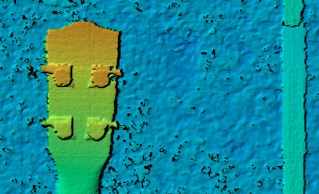
Up until now ODM was able to process only JPG files. With this release we added support for processing TIFF files, both 8bit and 16bit. TIFF is a popular format especially with multispectral and thermal cameras.

Mapir Camera 16bit TIFFs processed in ODM

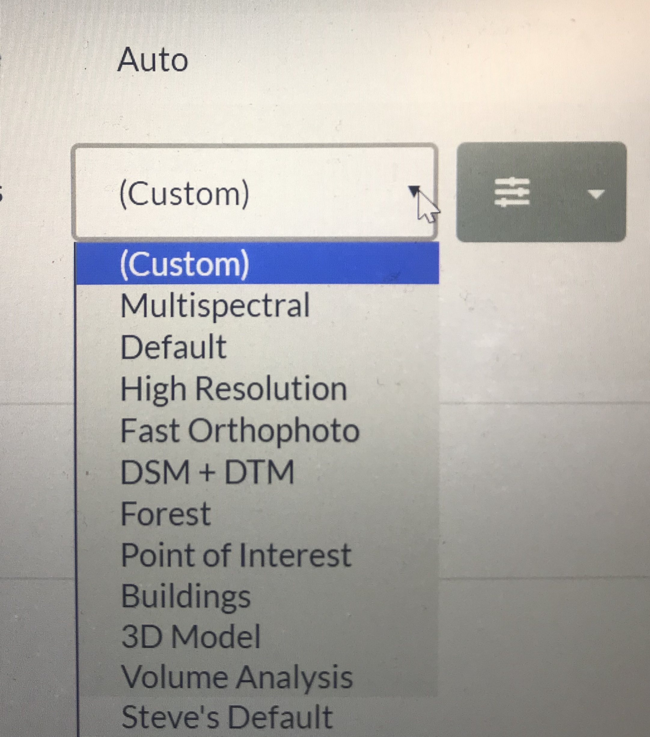
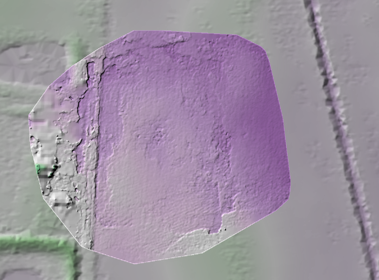
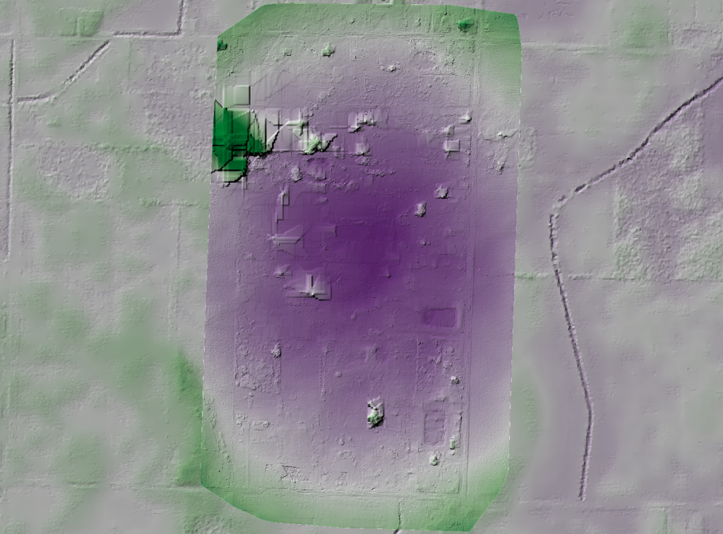
Multispectral Support (Experimental)

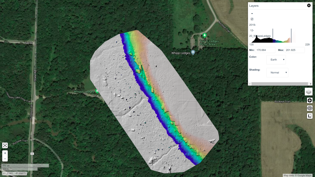
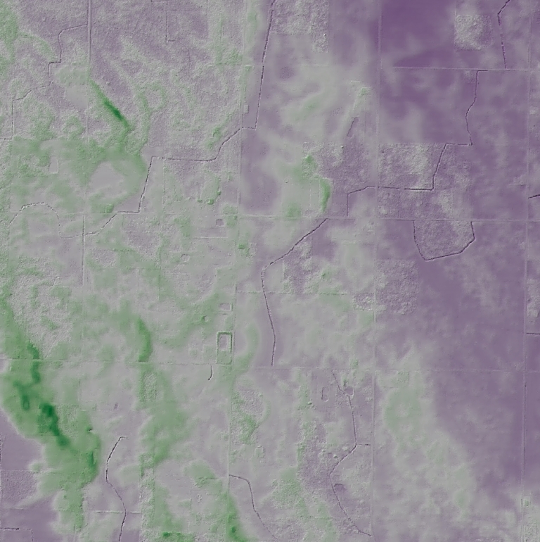
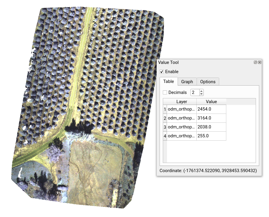
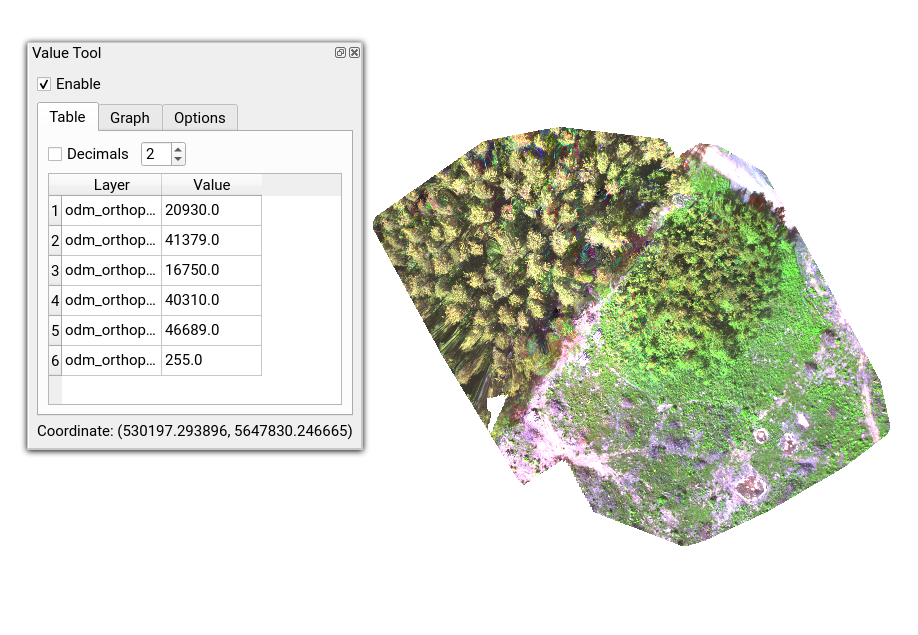
We have added the ability to process multispectral images (for example those captured with a Parrot Sequoia, MicaSense Altum or RedEdge). We have obtained some promising preliminary results. When provided with N camera bands, ODM will generate an N band orthophoto (in the proper bit resolution, up to 16).

We have not added support for spectral calibration targets, which we plan to add in the near future and we’re currently looking to add support for more cameras. The task of identifying different bands is different for each camera vendor and we’ll need to add support for more cameras with time. We hope the community will start to process some datasets and help us improve multispectral support (share your datasets?)

MicaSense RedEdge 5 Bands processed in ODM

We recommend to pass the –texturing-skip-global-seam-leveling option when processing thermal/multispectral datasets. Global seam leveling will attempt to normalize the values distribution across orthophotos, which works well for making pretty RGB images, but will affect measured values in thermal/multispectral settings.

Split-merge Improvements

We rewrote from scratch the orthophoto cutline blending algorithm to merge orthophotos, a bottleneck that was causing processing to take longer than necessary in the last stage of the pipeline. The new algorithm is faster and much more memory efficient. We also sped up by a factor of 30x the time it takes to merge point clouds from submodels, as well as reducing memory usage drastically.

OpenSfM/MVE Updates

We brought the latest version of OpenSfM in this update, which delivers up to 1.6x faster image matching than before.

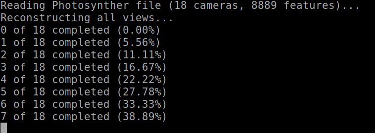
MVE has also been (finally) modified to report progress on the status of computations. You’ll finally know if the program is “stuck” or not.

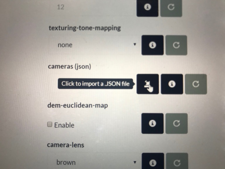
Improved Brown-Conrady Camera Model

We made modifications to the camera model used to compute camera poses and points. Up until now the default in ODM has been to use a simplified perspective camera model. The community has been testing the usage of the brown-conrady model for a while, with great results. The original brown-conrady model however uses two parameters for specifying focal length, which are unfortunately not accurately supported by the texturing and dense reconstruction stages of the pipeline (a single focal length is used by those stages). We’ve approximated the brown-conrady computation by averaging the two focal lengths, but could we do better? Yes!

We modified the brown-conrady model to use a single focal length, bringing the model to full support for all stages of the pipeline and set it as the default camera model. We expect this will improve the quality of results for all outputs. Preliminary tests confirm this.

EPrfdJAW4AAKQZW — Credits: Klas Karlsson

Easier To Contribute to ODM

If you are on Linux, it’s now easier than ever to make a change to ODM. A new script setups a development environment for you inside a docker container.

And One More Thing: NodeODM Changes

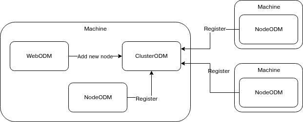
NodeODM now exposes a task list API endpoint. This is a feature that has been requested a lot and allows people to view the tasks running on a particular node. If you send a task to NodeODM via WebODM (or CloudODM or PyODM, or any other client), if you open the NodeODM interface you will be able to monitor and manage the task. This is also implemented in ClusterODM.

We have also replaced the .zip compression method in NodeODM to be faster, more memory efficient.

What do you think of the new changes? Try them out and report any bug.

Reconstructing cliffs in OpenDroneMap, or how to beat LiDAR at its own game

2020-02-02 (updated 2020-02-02)

From the top of Whipps Ledges at Hinckley Reservation on November 16, 2016 (Kyle Lanzer/Cleveland Metroparks)

Reposted from smathermather.com

LiDAR and photogrammetric point clouds

If we want to understand terrain, we have a pricey solution and an inexpensive solution. For a pricey and well-loved solution, LiDAR is the tool of choice. It is synoptic, active (and therefore usable day or night), increasingly affordable (but still quite expensive), and works around even thick and tall evergreen vegetation (check out Oregon’s LiDAR specifications as compared with US federal ones, and you’ll understand that sometimes you have to turn the LiDAR all the way up to 11 to see through vegetation).

For a comparably affordable solution, photogrammetrically derived point clouds and the resultant elevation models like the ones we get from OpenDroneMap are sometimes an acceptable compromise. Yes, they don’t work well around vegetation in thickets and forests, and other continuous vegetation covers, but with a few hundred dollar drone, a decent camera, and a bit of field time, you can quickly collect some pretty cool datasets.

As it turns out, sometimes we can collect really great elevation datasets derived from photogrammetry under just the right conditions. More about that in a moment: first let’s talk a little about the locale:

Sharon Conglomerate and Whipps Ledges, Hinckley Reservation

One of my favorite rock formations in Northeast Ohio is Sharon Conglomerate. A mix of sandstone and proper conglomerate, Sharon is a stone in NEO that provides wonderful plant and animal habitats, and not coincidentally provides a source of coldwater springs, streams, and cool wetland habitats across the region. A quick but good overview of the geology of this formation can be found here:

Visiting Sharon

Mapping conglomerate

One of the conglomerate outcrops in Cleveland Metroparks is Whipps Ledges in Hinckley Reservation. It’s a favorite NEO climbing location, great habitat, and a beautiful place to explore. We wanted to map it with a little more fidelity, so we did a flight in August hoping to see and map the rock formations in their glorious detail:

Overall orthophoto of Whipps Ledges from August 2019

Digital surface model of the forest over

Inset image of Whipps Ledges from August 2019

Inset digital surface model of the forest over

Unfortunately, as my geology friends and colleagues like to joke, to map out the conglomerate, we need to “scrape away the pesky green vegetation stuff first”. We don’t want to do this, of course — this is a cool ecological place because it’s a cool geological place! It just happens to be a very well vegetated rocky outcrop. The maple, beech, oak and other trees there take full advantage of the lovely water source the conglomerate provides, so we can’t even glean the benefits of mapping over sparse and lean xeric oak communities: this is a lush and verdant locale.

So yesterday, we flew Whipps Ledges again, but this time the leaves were off the trees. It can be a challenge still to get a good sense of the shape of the landform, even with leafless trees: forest floors do not provide good contrast with the trees above them, and it can be difficult to get good reconstructions of the terrain.

But yesterday, we were lucky: there was a thin layer of snow everywhere providing the needed contrast without being too thick to distort the height of the forest floor too much; shadows from the low sun created great textures on the featureless snow that could be used in matching.

Image above the snowy forest on Whipps Ledges

The good, the bad, and the spectacular

The bad…

So, how are the results? Let’s start with the bad. The orthophoto is a mess. There’s actually probably very little technically wrong with the orthophoto: the stitching is good, the continuity is excellent, the variation between scenes non-existent, the visual distortions minimal. But, it’s a bad orthophoto in that between the high contrast between the trees and the snow compounded with the shadows from the low, nearly cloudless sky result in a difficult to read and noisy orthophoto. Bad data for an orthophoto in; bad orthophoto out.

The good

The orthophoto wasn’t our priority for these flights, however. We were aiming for good elevation models. How is our Digital Terrain Model (DTM)? It’s pretty good.

Photogrammetrically derived digital terrain model from drone imagery

The DTM looks good on it’s own, and even compares quite favorably with a (admittedly dated, 2006) LiDAR dataset. It is crisp, shows the cliff features better than the LiDAR dataset, and represents the landform accurately:

Comparison of crisp and cliff-like OpenDroneMap digital terrain model and the blurry LiDAR dtm.

The spectacular

So, if the ortho is bad and the DTM is good, what is great? The DSM is quite nice:

Overview of digital Surface Model from December 21 flight

The DSM looks great. We get all the detail over the area of interest, each cliff face and boulder show up clearly in the escarpment.

Constraining the elevation range to just those elevation around the conglomerate outcrop.

Constraining the elevation range to just those elevation around the conglomerate outcrop , inset 1

Constraining the elevation range to just those elevation around the conglomerate outcrop , inset 2

Improvements in the next iteration

The digital surface model is really quite wonderful. In it we can see many of the major features of the formation, including named features like The Island, a clear delineation of the Main Wall and other features that don’t show in the existing terrain models.

Due to untuned filtering parameters, we filter out more of the features than we’d like in the terrain model itself. It would be nice to keep The Island and other smaller rocks that have separated from the primary escarpment. I expect that when we choose better parameters for deriving the terrain model from the surface model points, we can strike a good balance and get an even better terrain model.

Animation comparing digital surface model and digital terrain model showing the loss of certain core features to Whipps Ledges due to untuned filtering parameters in the creation of the terrain model.

Beating LiDAR at it’s own game

It is probably not fair to say we beat LiDAR at it’s own game. The LiDAR dataset we have to compare to is 13 years old, and a lot has improved in the intervening years. That said, with a $900 drone, free software, 35 minutes of flying, and two batteries, we reconstructed a better terrain model for this area than the professional version of 2006.

And we have control over all the final products. LiDAR filtering tends to remove features like this regardless of point density, because The Island and similar formations are difficult to distinguish in an automated fashion from buildings. Tune the model for one, and you remove the other.

For our use case, however, we can use the best parameters for this area, take a high touch approach, and create a really nice map of a special area in our parks for very low cost. High touch/low cost. I can’t think of a sweeter spot to reach.

Choosing good OpenDroneMap parameters

2020-01-31

Introduction

I had an interesting question recently at a workshop: “What parameters do you use for OpenDroneMap?” Now, OpenDroneMap has a lot of configurability, lots of different parameters, and it can be difficult to sift through to find the right parameters for your dataset and use case. That said, the defaults tend to work pretty well for many projects, so I suspect (and hope) there are a lot of users who never have to worry much about these.

The easiest way to proceed, is to use some of the pre-built defaults in WebODM. These drop downs let you take advantage of the combination of a few different settings abstracted away for convenience, whether settings for processing Multispectral data, doing a Fast Orthophoto, flying over Buildings or Forest, etc.

You can also save your own custom settings. You will see at the bottom of this list “Steve’s Default”. This has a lot of the settings I commonly tweak from defaults.

Back to the question at hand: what parameters do I change and why? I’ll talk about 7 parameters that I regularly or occasionally change.

The Parameters

Model Detail

Occasionally we require a little more detail (sometimes we also want less!) in our 3D models from OpenDroneMap. Mesh octree depth is one of the parameters that helps control this. A higher number gives us higher detail. But, there are limits to what makes sense to set for this. I usually don’t go any higher than 11 or maybe 12.

Elevation Models

DTM/DSM

Often with a dataset, I want to calculate a terrain model (DTM) or surface model (DSM) or both as part of the products. To ensure these calculate, we set the DTM and DSM flags. The larger category for DTM and DSM is Digital Elevation Model, or DEM. All flags that affect settings for both DTM and DSM are named accordingly.

Ignore GSD

OpenDroneMap often does a good job guessing what resolution our orthophoto and DEMs should be. But it can be useful to specify this and override the calculations if they aren’t correct. ignore-gsd is useful for this.

DEM Resolution

DEM Resolution applies to both DTMs and DSMs. A criterion that is useful to follow for this setting is 1/4th the orthophoto resolution. So, if you flew the orthophoto at a height that gives you 1cm resolution ortho imagery, your dem-resolution should probably be 4cm.

Depthmaps

Depthmap resolution

A related concept is depthmap resolution. Depthmaps can be thought of as little elevation models from the perspective of each of the image pairs. The resolution here is set in image space, not geographic coordinates. For Bayer style cameras (most cameras), aim for no more than 1/2 the linear resolution of the data. So if your data are 6000×4000 pixels, you don’t want a depthmap value greater than 3000.

That said, usually, 1/4 is a better, less noisy value, and depthmap calculations can be very computationally expensive. I rarely set this above 1024 pixels.

Camera Lens Type

I saved the best for last here. So, if you’ve made it this far in the blog post, this is the most important tip. In 2019, OpenSfM, our underlying Structure from Motion library, introduced the Brown-Conrady camera model as an option. The default for camera type is auto, which usually results in the use of a perspective camera, but Brown-Conrady is much better. Set your camera-lens to brown, and you will get much better results for most datasets. If it throws an error (which does happen with some images), just switch it back to auto and rerun. Brown will be a default in the near future.

SELF CALIBRATION OF CAMERAS FROM DRONE FLIGHTS (PART 3)

2019-12-06 (updated 2019-12-06)

BACKGROUND

(Reposted from https://smathermather.com/2019/12/02/self-calibration-of-cameras-from-drone-flights-part-3/)

I have been giving a lot of thought to sustainable ways to handle self calibration of cameras without undue additional time added to flights. For many projects, I have the luxury of spending a little more time to collect more data, but for larger projects, this isn’t a sustainable model. In a couple of previous posts (this one and this one), we started to address this question, pulling from the newly updated OpenDroneMap docs to highlight the recommendations there.

As I have been thinking about these recommendations, there are other more efficient ways to accomplish the same goal. Enter the calibration flight: the idea is that with some cadence, we have dedicated flights at the same height and flight speed as the larger flight in order to estimate lens distortion.

INITIAL TEST

For this testing, I chose a relatively flat but slightly undulating area in Ohio in the USA: the Oak Openings region, which is a lake bottom clay lens overlayed with sand dunes from glacial lakes. It has enough topography to be interesting, but is flat enough to be sensitive to poor elevation models.

Shaded elevation model in green and purple — Shaded elevation model of the Oak Openings region in Northwest Ohio, USA. Purple is lower elevations, green higher elevations, typically vestigial dunes. Elevation model from Ohio Statewide Imagery Program.

The test area flown is ~80 acres of residences, woodlots, and farmland.

Flown with a DJI Mavic Pro which has an uncalibrated lens with movable focus, the first question I wanted to address is how much distortion do we get in our resultant elevation models if we just allow for self calibration? It turns out, we get a lot:

Image showing bulls-eye pattern of lens distortion in digital terrain model with self calibrated approach — Bulls-eye pattern of lens distortion in digital terrain model with self calibrated approach

We have seen this in other datasets, but this forms a good baseline for our subsequent work to remove this.

Next step, we fly a calibration pattern. In this case, I plotted an area large enough to capture two passes of data, plus an orbit around the exterior of the area with the camera angled at 45° for a total of 3 minutes and 20 seconds.

Figure showing layout of calibration flight pattern — Layout of calibration flight pattern

When we process this data in OpenDroneMap, we can extract the cameras.json file (either in the processing directory or we can download from WebODM) and use that in another model. We can do this using the cameras parameter on the command line or in WebODM through uploading the json file from our calibration dataset.

Cameras option in WebODM for importing camera parameters

But, before we do that, let’s do a review of our calibration data — process it and take a look at what kind of output we get. First, we process it using defaults and evaluate the elevation model to look for artifacts that might indicated whether the calibration pattern wasn’t successful.

Our terrain model from the Ohio Statewide Imagery Program elevation model looks like this for our calibration area:

Shaded elevation model from Ohio Statewide Imagery program for calibration area

Note that this is mostly a moderately flat farm field with a road and small ditches running North/South in the west of the image and a deep Northeast Ohio Classic ditch in the east.

How does our data from our calibration flight look?

Image showing elevation model from calibration flight — Elevation model from calibration flight

It’s not bad. We can see the basic structure of the landscape — from the road in the west to the gentle drop in elevation in the east.

Our default camera model is a perspective camera. How does this look with the Brown–Conrady camera model that Mapillary recently introduced into OpenSfM?

Image showing elevation model from calibration flight with Brown camera model — Elevation model from calibration flight with Brown–Conrady camera model

With the Brown–Conrady camera model, we see additional definition of the road bed, ditches alongside the road, and even furroughs that have been ploughed into the field. For this small area, it appears the Brown–Conrady camera model is really improving our overall rendering of the digital terrain model, likely as a result of an improved structure from motion product. We even see the small rise in the field at the southern central part of the study area, and as with the default (perspective) model, the slope down toward the ditch on the east of the study area.

RESULTS

With running these both with perspective and Brown–Conrady cameras, we can apply those camera models as fixed parameters for our larger area and see what kind of results we get.

Figure of larger elevation model as processed with perspective camera parameters as compared with reference model — Larger elevation model as processed with perspective camera parameters as compared with reference model

Our absolute values aren’t correct (which we expect), but the relative shape is — the dataset is now appropriately relatively flat with clear delineation of some of the sand features. This is the goal, and we have achieved it with some of the most challenging data.

How does our Brown–Conrady calibration model turn out? It did so well on the small scale, will we see similar results over the larger area?

Figure of larger elevation model as processed with brown camera parameters showing bulls-eye pattern — Larger elevation model as processed with Brown–Conrady camera parameters

In this case, no: the Brown–Conrady model over compensates for our distortion parameters. More tests need to be done in order to understand why. For now, I recommend using the perspective model for corrections on large datasets, and Brown–Conrady camera model on smaller datasets where the details matter, but the distortion isn’t discernible.

Self Calibration of Cameras from Drone Flights

2019-09-25 (updated 2019-09-24)

(Modified excerpt from the OpenDroneMap docs)

Calibrating the Camera

Camera calibration is a special challenge with commodity cameras. Temperature changes, vibrations, focus, and other factors can affect the derived parameters with substantial effects on resulting data. Automatic or self calibration is possible and desirable with drone flights, but depending on the flight pattern, automatic calibration may not remove all distortion from the resulting products. James and Robson (2014) in their paper Mitigating systematic error in topographic models derived from UAV and ground‐based image networks address how to minimize the distortion from self-calibration.

image of lens distortion effect on bowling of data

Bowling effect on point cloud over 13,000+ image dataset collected by World Bank Tanzania over the flood prone Msimbasi Basin, Dar es Salaam, Tanzania.

To mitigate this effect, there are a few options but the simplest to flight plan are as follows: fly two patterns separated by 20°, and rather than having a nadir (straight down pointing) camera, use one that tilts forward by 5°.

As this approach to flying can be take longer than typical flights, a pilot or team can fly a small area using the above approach. OpenDroneMap will generate a calibration file called cameras.json that then can be imported to be used to calibrate another flight that is more efficiently but, from a self calibration perspective, less accurately.

Vertically separated flight lines with the above interleaved 20° flight pattern also improve accuracy, but less so than a camera that is forward facing by 5°.

figure showing effect of vertically separated flight lines and forward facing cameras on improving self calibration

From James and Robson (2014), CC BY 4.0

Kole Wetland Canal Mapping with ClusterODM

2019-09-20 (updated 2019-09-20)

Our friends and collegues at International Center for Free and Open Source Software in Kerala, India have done a pretty interesting and massive mapping initiative over Thrissur Kole Wetlands. The wetlands are a massive 30,000+ acre area that are both important to wildlife and provide rice production.

Suman Rajan, Asish Abraham, and Deepthi Patric (left to right in image below) mapped 9000 acres of it.

Given the massive scale of the project, they ran it across multiple nodes using a cluster of computers coordinated by ClusterODM.

What a beautiful cluster, and an important and interesting project.

Toward ODM 1.0 and Beyond

2019-09-09 (updated 2019-09-09)

During this past summer, the OpenDroneMap team has been active on a number of fronts.

Split-Merge Improvements

While this feature has been announced months ago, we’ve been working on a number of improvements to make it more stable and fast. The distributed split-merge workflow in particular is non-trivial and has required a number of fixes to improve its reliability over time. The LocalRemoteExecutor (LRE) module is perhaps one of the most interesting modules in the codebase, allowing submodels to be processed with a mix of local and remote processing, working in sync with ClusterODM (which is now more fault tolerant).

Ground Control Points

GCPs kept confusing our users with respect to supported coordinate reference systems (CRS). The system only handled well UTM CRSes, but the software happily accepted others, some which worked, some which didn’t.

If you are a frequent user on our forum you might have noticed a significant decrease (disappearance?) of questions related to GCPs. That’s because without fanfare, we’ve improved significantly GCP support in July (see PR #997). You can now use whatever CRS you please and ODM will handle the rest.

Major Speed Improvements

Our friends at Mapillary have also been working throughout the summer and brought some really neat new features to OpenSfM. Among some of these, there’s Bag of Words (BoW) matching, which significantly boosts reconstructions lacking georeferencing information. Datasets captured with a handheld camera are now much faster to process. You will also notice speed-ups for processing normal drone datasets (unrelated to BoW matching).

Camera Calibration Transfer and Models

Up until recently, you might have had some difficulty processing datasets captured with fisheye cameras such as the ones found in GoPros or Parrot Bebop drones.

ODM now comes with support for 4 different camera models:

Perspective (default)
Brown (like perspective, but capable of handling more complex distortion models)
Fisheye
Equirectangular (spherical)

To use a particular camera model simply pass –camera-lens <type> (lower case).

Bebop dataset before latest changes. Problem?

Processed by passing **–camera-lens fisheye**. Better!

It’s also possible to transfer a camera calibration model computed from one dataset to process another. This is useful to process a dataset that was captured in less-than-ideal conditions (for which good camera calibration parameters cannot be computed), but for which a good dataset captured with the same camera exists.

A cameras.json file is now created and placed in the root folder of each project and that file can be reused to process another dataset via –cameras /path/to/cameras.json.

Automated Docker Builds

Since ODM takes a while to compile, we haven’t been able to leverage Docker Hub’s ability for automatic builds (due to system timeouts). So up until a few days ago we have been building and publishing docker images manually. But no more! Starting from last week, a dedicated build server checks for changes on the ODM and WebODM repositories and automatically builds, tags and pushes the latest changes in master to Docker Hub.

ODM Book

Last but not least, the first edition of OpenDroneMap: The Missing Guide has been published. Spanish and Portuguese translations are also on the way. This has been a very time consuming task, but one which we hope will help more people get the most out of OpenDroneMap.

Future Plans

The community has already provided tremendous feedback. We know what needs to be done and we will continue to listen to our users. Among some of the most requested features:

Better GCP interface / workflows
Quality/Accuracy reports
Override mechanism for EXIF coordinates (PPK)
Multiband (TIFF) image support
NDVI, VARI index support (and others)
WebODM interface/workflow improvements

If your organization uses OpenDroneMap and is in a position to help (financially or by dedicating a developer to a task), get in touch on the forum.

Stitching Historical Aerial Images From 1940 Using OpenDroneMap

2019-05-17 (updated 2019-05-17)

During the recent OSGeo Code Sprint hosted at the University of Minnesota, we had the opportunity to learn more about the university’s effort to preserve some historical archives of aerial imagery.

We put our eyes on an old 1940 dataset of Hennepin County, Minnesota. The images are overlapping by about 20-30%. There’s also paper tears in many of the scans. We had never tried this before. Would it be good enough for ODM to process? We had to find out.

We quickly put together a script to download some of the images from the University’s online archive, add EXIF tags to the images and send them to ODM using the –fast-orthophoto option, which works well for high altitude flights and datasets with little overlap. We didn’t know what to expect. But a few hours later, when we saw the results, we knew it had worked!

Code available at: https://github.com/pierotofy/historical_aerial_downloader

GeoTIFF: https://drive.google.com/open?id=18UhkAR5jggOtgNvBzadEz-P-bymu14_m

Images credits to the University of Minnesota.

Parallel Shells: distributing split-merge with ClusterODM

2019-05-15 (updated 2019-05-15)

Code/community sprints are a fascinating energy. Below, we can see a bunch of folks laboring away at laptops scattered through the room at the OSGeo’s 2019 Community Sprint, an exercise in a fascinating dance of introversion and extroversion, of code development and community collaboration.

A portion of the OpenDroneMap team is here for a bit working away at some interesting opportunities. Tonight, I want to highlight an extension to work mentioned earlier on split-merge: distributed split-merge. Distributed split-merge leverages a lot of existing work, as well as some novel and substantial engineering solving the problem of distributing the processing of larger datasets among multiple machines.

Image of the code sprint.

This is, after all, the current promise of Free and Open Source Software: scalability. But, while the licenses for FOSS allow for this, a fair amount of engineering goes into making this potential a reality. (HT Piero Toffanin / Masserano Labs) This also requires a new / modified project: ClusterODM, a rename and extension of MasseranoLabs NodeODM-proxy. It requires several new bits of tech to properly distribute, collect, redistribute, then recollect and reassemble all the products.

Piero Toffanin with parallel shells to set up multiple NodeODM instances

————————————————————————————————–

“Good evening, Mr. Briggs.”

The mission: To process 12,000 images over Dar es Salaam, Tanzania in 48 hours. Not 17 days. 2 days. To do this, we need 11 large machines (a primary node with 32 cores and 64GB RAM and 10 secondary nodes with 16 cores and 32GB RAM), and a way to distribute the tasks, align the tasks, and put everything back together. Something like this:

… just with a few more nodes.

Piero Toffanin and India Johnson working on testing ClusterODM

This is the second dataset to be tested on distributed split-merge, and the largest to be processed in OpenDroneMap to a fully merged state. Honestly, we don’t know what will happen: will the pieces process successfully and successfully stitch back together into a seamless dataset? Time will tell.

For the record, the parallel shells were merely for NodeODM machine setup.

Actually distributing the jobs? Easy:

Split-merge nearing completion

2019-05-01 (updated 2019-05-01)

For anyone using OpenDroneMap to process really large datasets, some good news came through early last year with improvements to how OpenSfM handles large datasets. This came in the form of an innovative, first of it’s kind, hybrid SfM method which combines the better attributes of global and incremental SfM approaches.

TLDR: This helps make processing large datasets orders of magnitude faster, and can be tuned to be even faster (at some accuracy expense), which is really exciting and wonderful work by the folks (especially Pau) over at Mapillary.

But this change was not enough for OpenDroneMap. After the SfM step, we have several more processing steps, all challenges with respect to data processing techniques, memory usage, and other issues which crop up when you adapt a bunch of libraries meant for one thing to another set of much larger things.

Enter: split-merge. Since early last year, we have also had some scripts to help split up large datasets into smaller pieces, keeping those smaller pieces aligned with each other, and helping with some of the merging of those data back into a cohesive whole at the end. This was a great work-around for processing those larger datasets, but for a variety of reasons (funding and time being the big two), never got completed.

Now a big phase of that work is wrapping up. You can find that work in Pull Request #979. Do you have a really large dataset that needs processing on the ODM command line? Try the following:

./run.sh --project-path /path/to/datasets --split <target number of pictures per submodel> mydataset

Coming soon to a WebODM near you… .

(HT Pau Gargallo Piracés at Mapillary, Dakota Benjamin at Humanitarian OpenStreetMap Team, and Piero Toffanin at Masserano Labs)